45 conditional formatting pivot table row labels

Design the layout and format of a PivotTable Right-click the field name and then select the appropriate command — Add to Report Filter, Add to Column Label, Add to Row Label, or Add to Values — to place the field in a specific area of the layout section. Click and hold a field name, and then drag the field between the field section and an area in the layout section. Pivot Table Conditional Formatting - Contextures Excel Tips This step will prevent conditional formatting problems after you refresh the pivot table. Select any cell in the pivot table On the Ribbon's Home tab, click Conditional Formatting, then click Manage Rules The Conditional Formatting Rules Manager opens, where you can create a new rule, edit an existing rule, or delete a rule

How to Apply Conditional Formatting to Pivot Tables So in this post I explain how to apply conditional formatting for pivot tables. 1. Select a cell in the Values area The first step is to select a cell in the Values area of the pivot table. If your pivot table has multiple fields in the Values area, select a cell for the field you want to apply the formatting to. 2. Apply Conditional Formatting

Conditional formatting pivot table row labels

Excel Pivot Table Conditional Formatting Row Labels Go making the conditional formatting select the color scale and do it based on commercial and choose diverging and the colors should give expected result. Here a glaze color or bar and been applied... Conditional Formatting PivotTables - My Online Training Hub Here's a step by step how to: 1. Select any cell in the values area of your PivotTable. 2. On the Home tab of the Ribbon select Conditional Formatting > Top/Bottom Rules > Top 10 Items: 3. Set the value to 1 and choose your format: 4. You will now have an icon beside the cell that you have applied the formatting to. Apply Conditional Formatting | Excel Pivot Table Tutorial Go to Home Tab → Styles → Conditional Formatting → New Rule. From rule to, select the third option. And, from "select a rule" type select "Format only top or bottom" ranked values. In edit rule description, enter 1 in the input box and from the drop-down menu select "each Column Group". Apply formatting you want. Click OK.

Conditional formatting pivot table row labels. Pivot Table with Conditional Formatting - Microsoft Community Ok, Pivot Tables are good, Pivot Tables are our friends. Now I want to use conditional formatting with a pivot table. I have seen a lot of examples, but none showing me how to use a field in the field list in the formula of a conditional format. Perhaps this is not possible, so I moved the field into a row label. Conditional formatting rows in a pivot table based on one rows criteria ... What you need to do is accept the formula the way you type it, close the conditional formatting rules manager and then reopen it. Remove the $ from the row numbers that excel added into your formula but leave it on the column number like so =$I3=992, or whatever your first row is. Pivot Table: Pivot table conditional formatting - Exceljet Select any cell in the data you wish to format and then choose "New rule" from the conditional formatting menu on the Home tab of the ribbon. At the top of the window, you will see setting for which cells to apply conditional formatting to. For the example shown, we want: "All cells showing sum of "sales values" for name and "date" Copy conditional Formatting to all rows of Pivot Table I have a pivot table that has a row of 5 columns with sales results in each. I set up a conditioning format that shows the cells in that row that exceed the average. My question is how do I copy this formatting to all the rows below without having to enter the same formula for each row. Thanks so much for your help and time..KH.

Excel Conditional Formatting in Pivot Table - EDUCBA Click on any cell in the pivot table > Go to the HOME tab > Click on Conditional Formatting option under Styles option > Click on Manage Rules option. It will open a Rules Manager dialog box. Click on the Edit Rule tab, as shown in the below screenshot. It will open the Editing Rule formatting window. Refer to the below screenshot. Conditional Formatting on Pivot Table row labels In srcFromPowerPivot sheet cell A is from powerpivot under row label comparing the dates in cell C (3 dates) and the condtional formatting doesnt work. In cell J it worked cos I dragged under value instead of row label. In the srcFromWorksheet it worked even though it is under rowlabel. Sheet3 is just a copy of powerpivot data. Pivot Table Grouping, Ungrouping And Conditional Formatting So let's drag the Age under the Rows area to create our Pivot table. #1) Right-click on any number in the pivot table. #2) On the context menu, click Group. #3) Grouping dialog box appears, in this example, the least number is 25, so by default the Starting number is entered as 25, and you can change if necessary. Pivot Table Conditional Formatting with VBA - Peltier Tech Without resorting to macros, it's possible to quickly reapply the conditional format in 2007 by following these steps: - Set the conditional format to range covering more than the pivot table (e.g. on cell above). - When the pivot is refreshed, go to the "Conditional formatting Manage Rules…" dialog and edit the "Applies to" range.

Format Pivot Table Labels Based on Date Range Select all the dates in the Row Labels that you want to format. On the Ribbon, click the Home tab, and then in the Styles group, click Conditional Formatting. In the list of conditional formatting options, click Highlight Cells Rules, and then click A Date Occurring. In the date range drop-down, select Next Month, and then click the arrow to ... Conditional formatting for Pivot Tables in Excel 2016 - Ablebits Conditional formatting when applied to PivotTables in Excel 2007 - 2016 is applied to the underlying structure of the PivotTable rather than to the cells themselves. So, when you interact with a PivotTable such as moving fields around and viewing your data in different ways, the formatting is updated as you work. Conditional Formatting in Pivot Table - WallStreetMojo We must follow the steps to apply conditional formatting in the pivot table. First, we must select the data. Then, in the "Insert" Tab, click on "Pivot Tables." As a result, a dialog box appears. Next, we must insert the pivot table in a new worksheet by clicking "OK." Currently, a pivot table is blank. Next, we need to bring in the values. Conditional Format Pivot Table Row - Chandoo.org Select the entire row, and when you apply the conditional format, make the column reference absolute. So, say we want the entire row 2 to be formatted if cell in col B = 5. formula would be: =$B2=5

34 Using The Current Worksheets Pivot Table Add The Task Name As A Column Label - Labels ...

conditional formatting per row on pivot - Microsoft Tech Community conditional formatting per row on pivot. Hi, I would like to format each row of a pivot table separately (as in the picture shown below), but I cannot paste the formatting. I've got many rows, and they could change (just like the columns)

pivot table - Conditional formatting between 2 sheets - Super User

Pivot table conditional format based on row value - Chandoo.org In the picture below you can see I have grouped some values together to form the row categories - I would like to tell excel to fill the cells with the data a different color where the row is "600-650" and a different color again for the row value "550-600" and so on for all the row categories shown.

How to Apply Conditional Formatting in Pivot Table? (with Example)

How to Apply Conditional Formatting to Rows Based on Cell Value On the Home tab of the Ribbon, select the Conditional Formatting drop-down and click on Manage Rules…. That will bring up the Conditional Formatting Rules Manager window. Click on New Rule. This will open the New Formatting Rule window. Under Select a Rule Type, choose Use a formula to determine which cells to format.

Sorting a Pivot Table | MyExcelOnline

Above Average Conditional Formatting in Pivot Table off Row Total This is inverted from a normal pivot table where the months are usually the row labels. Basically I want the table to look at the value in the Values cells to look at the row Average instead of the column Average. Is there a way to do this? I've highlighted all my Value cells (showing the sum of the issue for a specific month) and then applied ...

Create Beautiful Reports with Custom Pivot Tables and JavaScript Spreadsheets | SpreadJS

Excel VBA: Conditional Format of Pivot Table based on Column Label myPivotSourceName = myPivotField.Name. Then rather than referencing the data field with the pivot field object, I referenced the DataRange with the string: myPivotTable.PivotFields (myPivotSourceName).DataRange.Select. Works perfectly and is completely portable for any pivottable on any sheet with any fields. excel vba.

Finding Duplicates by Using Conditional Formatting in Excel 2010

Pivot Table Conditional Formatting for Different Rows Items? Hello, It is possible! All you have to do: Select Your Pivot Table and: Go to Conditional Formatting -> New Rule -> Choose All cells showing "duration" values for "Type and "Date Selection" under "Apply Rule To" section -> Use a Formula to Determine which cells to format and enter the following formula: =AND(A6="Cars",A6>3), You can create new rules for other two conditions as well:

Using column label as formatting condition in excel pivot table - Stack Overflow

How to rename group or row labels in Excel PivotTable? - ExtendOffice 1. Click at the PivotTable, then click Analyze tab and go to the Active Field textbox. 2. Now in the Active Field textbox, the active field name is displayed, you can change it in the textbox. You can change other Row Labels name by clicking the relative fields in the PivotTable, then rename it in the Active Field textbox.

How to repeat row labels for group in pivot table?

How to apply conditional formatting to Pivot Tables - SpreadsheetWeb Go to HOME > Conditional Formatting > New Rule to add a new formatting rule, or select from predefined options. If you select the latter, you will need to configure the rule regardless. The New (or Edit) Formatting Rule window contains options specific to Pivot Tables. You can choose the location where you want to apply your conditional ...

Pivoting-tour

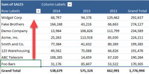
Issue with conditional formatting in pivot table - My Online Training Hub I made a pivot table to present three years data and highlighted the numbers > 249 with conditional formatting in the pivot table. ... i.e. not PivotTable conditional formatting. Apply it to the column, where the row label contains 'Total'. If you get stuck, please start a new thread as it will be off topic. Mynda. Forum Timezone: Australia ...

Learn How to Apply Conditional Formatting in a Pivot Table | Excelchat

Apply Conditional Formatting | Excel Pivot Table Tutorial Go to Home Tab → Styles → Conditional Formatting → New Rule. From rule to, select the third option. And, from "select a rule" type select "Format only top or bottom" ranked values. In edit rule description, enter 1 in the input box and from the drop-down menu select "each Column Group". Apply formatting you want. Click OK.

How To Find And Remove Duplicates In A Pivot Table - MS Excel | Excel In Excel

Conditional Formatting PivotTables - My Online Training Hub Here's a step by step how to: 1. Select any cell in the values area of your PivotTable. 2. On the Home tab of the Ribbon select Conditional Formatting > Top/Bottom Rules > Top 10 Items: 3. Set the value to 1 and choose your format: 4. You will now have an icon beside the cell that you have applied the formatting to.